Edward Taylor
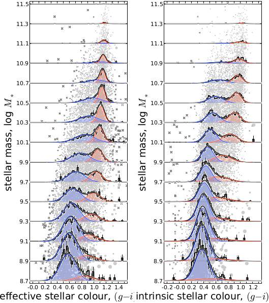
Demonstrating the quality of our fits to the joint colour–mass distributions.— The histograms in each panel show the incompleteness-corrected distribution of colours of z < 0.12 galaxies, computed in bins of log M∗ centred on log M∗ = 8.8, 9.0, …, 11.4. The left panel is for the effective (g-i) colour; the right panel is for the intrinsic, dust-corrected, stellar colour, (g-i)*. The errorbars show the statistical uncertainties on each these distributions, derived by bootstrap resampling. The smooth curves show the results of our modelling: the blue and red curves show the fit distributions for the B- and R-populations; the black curves shows the net B+R distributions. Underlaid beneath all this, the grey points show the data themselves; the size of each point reflects the relative 1/Vmax scaling used to account for selection effects. Note that we have not binned the data in the course of the fits; the binning in this Figure is for illustrative purposes only. It is clear that the fit model provides an excellent description of the observed data.
These two panels are the showpiece of a new study that i have spent the last 3 years (!!) working on, looking into the idea of ‘bimodality’ among galaxies. I have just (finally!) submitted this work to MNRAS; the paper is actually the first in a series of 5 in which i am developing a phenomenological description of the main stages of galaxy evolution.
The observational result of ‘bimodality’ has played a crucial role in the development of our theoretical understanding of the process of galaxy formation and evolution. Let me explain how, as briefly as i can.
It seems that there are two and only two kinds of galaxies: red ones, and blue ones. (This is, of course, an over simplification – in fact, it is exactly this kind of oversimplification that i am trying to bust! But it is fair to say that this is how a lot of people in the field talk about things, even if they don’t really believe it.) In simple terms, a blue colour implies that a galaxy has formed at least some stars in the past few hundred million years. A red colour can mean one of two things: it can mean either a very old stellar population, with no star formation over the past billion years or so, or it can mean that there is a lot of dust in the galaxy. (Dust makes things red: think about a sunset on a smoggy evening.) So - modulo dust - the difference between red and blue is the difference between ‘star-forming’ and ‘dead’
The weird thing is that the most massive galaxies tend to be red and dead. This is weird because gravity is what drives star formation. Naively, you might think that more mass means more gravity, and so more star formation. But that’s not what happens: apparently, there is something that kills or ‘quenches’ the process of star formation in massive galaxies. Nobody knows what this might be, even though this quenching problem is one of the most intensively studied areas of extragalactic astronomy over the last ten or twelve years.
Models of galaxy evolution have to include some ad hoc prescription for when star formation is quenched, but pretty much every model has its own prescription – no one really understands what the real physical mechanism is. As ridiculous as it sounds, the best way to constrain these models is simply to measure the relative and absolute numbers of ‘red’ and ‘blue’ galaxies.
Even more ridiculously, even after ten or twelve years, no one has really measured this well. Let me explain what i mean by that.
What people have done in the part (with only one notable exception, in 2004) is simply to draw a line that divides ‘red’ galaxies from ‘blue’ ones. The problem with this is that if you draw a different line, you get a different answer. And the decision about precisely where to draw the line is always arguable, hence arbitrary. This is even worse than it sounds: different choices for the line give you qualitatively different measurements.
So what I have done is to develop a mixture modelling approach. Instead of drawing a line to separate ‘red’ and ‘blue’ galaxies, I model the data as a mixture of two distinct but overlapping populations. This lets me figure out the number of galaxies in the ‘red’ and ‘blue’ populations without ever specifying whether any particular galaxy belongs to which population. This lets me get around the problem of having to draw a line – in fact, it gives a way to derive an objective, phenomenological classification scheme that is based on the data.
These plots show just how good a description of the data the mixture modelling provides.
What’s more, in the ‘intrinsic’ plot, I have actually performed a correction for dust, so that I really am distinguishing galaxies based on their stars, not just their apparent colours. And even better than that, although this point isn’t visually emphasised in the plots I’ve submitted, i get the same answer in both cases. In other words, if you do the mixture modelling well, you get the right answer, no matter whether you do the dust correction or not – I have definitely gotten around the dust problem. And that’s pretty neat.
The only other thing that I’ll say is that I had to learn a lot of statistics in order to do all this. The fits shown in each panel have 35-40 parameters (having done the full and proper Bayesian model selection to make sure that these really are the best and simplest descriptions of the data). This is a level of statistical rigor that is very, very rare in the field. But it is, in my opinion the way forward in the new age of ‘big data’ astronomy.
That was a lot of background, but i hope it wasn’t too painful to read!
There are two json archives that contain the data
for each of the two panels. There is also the script bimix.py that
should use these data to make the two plots. You can either (i hope!)
just python bimix.py at the command line, or run bimix.makePlots()
in interactive mode.
#! /usr/bin/env python
import numpy as np
from matplotlib import pyplot as p
import json
import os, sys, random, time
bluecolor = ( 0, .185, 1, 1 )
redcolor = ( 1, .185, 0, 1 )
masslimit = 8.7
def plotFitDistros( parVec, argList, figure=1, figsize=(4,9), figstring=None,
nbins=64, scaleby=0.765, massbin=0.2, massbins=None,
showdata=True, showbad=True, scalepoints=True,
applyerrors=True,
nowhite=False, bootstraps=200, printthings=False,
xlim=[8.675, 11.525], ylim=(-0.25, 1.45),
xlabel='stellar mass, log $M_*$',
ylabel='intrinsic stellar colour, $(g-i)_*$ ',
bestfit=False, logyblue=False,
redcolor=redcolor, bluecolor=bluecolor,
):
# compute the best fit (or whatever) model from parVec
( xobs, yobs, xerr, yerr, xycovar, weights, redlike, bluelike, badlike,
bluem, pblue, redm, pred, bluem1, pblue1, redm1, pred1,
bluem2, pblue2, redm2, pred2, bluey, bluedy, redy, reddy, result ) \
= bivarModel( parVec, *argList, returnFullModel=True, plotprob=0 )
goodlike = redlike + bluelike
if yerr.shape != yobs.shape : applyerrors = False
# open the figure
p.figure( figure, figsize=figsize ) ; p.clf()
p.subplots_adjust( left=0.22, right=0.95, top=0.995, bottom=0.065 )
# define point sizes, colors, etc.
if scalepoints :
psize = 2. + 1./weights * 2.
else :
psize = 8
pcolor= p.cm.gray_r( 0.2 )
palpha= 1.
bsize = 68. * np.clip( badlike / ( badlike + goodlike ), 0., 1. )**2.
# plot the datapoints
if showdata :
if showbad :
p.scatter( yobs, xobs, bsize, 'k', marker='x', zorder=-10 )
p.scatter( yobs, xobs, psize, pcolor, alpha=palpha,
edgecolors='none', zorder=-9 )
# p.xlim( ylim ) ; p.draw()
# define the mass bins in which histograms will be plotted
if massbins == None :
massbins = np.arange( masslimit, 11.5+massbin, massbin )[ ::-1 ]
# print massbins
# setup for showing the fit curves
ytp = np.linspace( ylim[0], ylim[1], nbins*4 )
densenorm = np.sum( 1 / weights )
# now, for each bin ...
for mi, m0 in enumerate( massbins ):
# ... select the galaxies that fall in this bin
inbin = np.where( np.abs( xobs - m0 - massbin/2. ) < massbin/2. )
# histograms for the observed data
hist, cedges = np.histogram(
yobs[inbin], weights=1./weights[inbin], range=ylim, bins=nbins )
pbins = ( cedges[:-1] + cedges[1:] ) / 2.
cbinwidth = cedges[1]-cedges[0]
hist = hist.astype( 'f' ) / densenorm / cbinwidth * scaleby
# will be plotted later
# bootstrapping to find statistical errors, if necessary
histerr = np.zeros( (2, pbins.shape[0]) )
if bootstraps <= 0 :
hihist = hist
lohist = hist
else :
bootvalues = np.zeros( (pbins.shape[0], bootstraps) )
binpop = len( inbin[0] )
# print binpop
for bi in xrange( bootstraps ):
if bi == 0 :
choices = inbin
else :
scores = ( np.random.rand( binpop ) * binpop ).astype( 'i' )
choices = inbin[0][ scores.ravel() ]
boothist, cedges = np.histogram(
yobs[choices], weights=1./weights[choices],
range=ylim, bins=nbins )
bootvalues[ :, bi ] = boothist
nz = np.where( boothist != 0 )
bootvalues = bootvalues.astype( 'f' ) / densenorm / cbinwidth * scaleby
counter = np.linspace( 0., 1., bootstraps )
percentiles = [ 0.158655, 0.841345 ]
for pi in range( pbins.shape[0] ):
sorted = np.argsort( bootvalues[ pi, : ] )
histerr[ :, pi ] = np.interp( percentiles, counter,
bootvalues[ pi, sorted ] )
hihist = histerr[ 1, : ]
lohist = histerr[ 0, : ]
if applyerrors :
# figure out how to deal with the observational errors
redweight = ( redlike / yerr*2 / weights )[ inbin ]
reddymean = np.sum( redweight * yerr[inbin] ) \
/ np.sum( redweight )
blueweight = ( redlike / yerr*2 / weights )[ inbin ]
bluedymean = np.sum( redweight * yerr[inbin] ) \
/ np.sum( redweight )
# figure out how to show the fits themselves
sumover = np.where( np.abs( redm - m0 - massbin/2. ) < massbin/2. )[0]
rxtp = np.zeros( ytp.shape )
bxtp = np.zeros( ytp.shape )
for mj in sumover:
rednorm= pred[ mj ]
redcen = redy[ mj ]
redvar = reddy[mj ]**2
if applyerrors : redvar += reddymean**2.
rxtp += rednorm / np.sqrt( 2. * np.pi * redvar ) \
* np.exp( -0.5*(ytp - redcen)**2 / redvar )
bluenorm= pblue[ mj ]
bluecen = bluey[ mj ]
bluevar = bluedy[mj ]**2.
if applyerrors : bluevar += bluedymean**2.
bxtp +=bluenorm / np.sqrt( 2. * np.pi *bluevar ) \
* np.exp( -0.5*(ytp - bluecen)**2 /bluevar )
# print redm[ mj ]
# print 'red :', np.sum(rxtp)/np.sum(rxtp+bxtp), redcen,np.sqrt( redvar)
# print 'blue :', np.sum(bxtp)/np.sum(rxtp+bxtp),bluecen,np.sqrt(bluevar)
rxtp *= massbin * scaleby / sumover.shape[0]
bxtp *= massbin * scaleby / sumover.shape[0]
# print 'red :', np.sum(rxtp)/np.sum(rxtp+bxtp), redcen,np.sqrt( redvar)
# print 'blue :', np.sum(bxtp)/np.sum(rxtp+bxtp),bluecen,np.sqrt(bluevar)
if not nowhite :
# fill in white under curves for this bin
p.fill_between( ytp, m0+0*ytp, m0+rxtp+bxtp, color='w', zorder=mi-0.8 )
p.fill_between( pbins, m0+0*hihist, m0+hihist, color='w', zorder=mi-0.8 )
# replot data points as necessary
limit1 = np.interp( yobs, ytp, m0+rxtp+bxtp )
limit2 = np.interp( yobs, pbins, m0+hihist )
limit = np.where( limit1 > limit2, limit1, limit2 )
replot = np.where( ( xobs > m0 ) & ( xobs < limit ) )
if len( replot[0] ) and showdata :
p.scatter( yobs[replot], xobs[replot], psize[replot], pcolor,
alpha=palpha, edgecolors='none', zorder=mi-0.7 )
# fill in under the fit curves
for ( xtp, ctp ) in zip( ( rxtp, bxtp ), ( redcolor, bluecolor ) ):
sig = np.where( xtp > 1e-4 )
p.fill_between( ytp[ sig ], m0 + 0.*xtp[ sig ],
m0+xtp[ sig ], color=ctp, alpha=0.2, zorder=mi-0.6 )
# plot the statistical uncertainties from bootstrapping
if bootstraps >= 0 :
for pi in np.where( hist > 0 )[0] :
p.plot( pbins[pi] * np.ones(2), [ m0+lohist[pi], m0+hihist[pi] ],
'w-', lw=2.4, zorder=mi-0.5 )
p.plot( pbins[pi] * np.ones(2), [ m0+lohist[pi], m0+hihist[pi] ],
'k-', lw=0.8, zorder=mi )
# plot the histograms for the data
p.plot( pbins, m0+hist, 'w-', lw=4, drawstyle='steps-mid', zorder=mi-0.5 )
p.plot( pbins, m0+hist, 'k-',lw=1.65,drawstyle='steps-mid',zorder=mi )
# actually show the fits
for ( xtp, ctp, lw ) in zip( ( rxtp + bxtp, bxtp, rxtp ),
( 'k', bluecolor, redcolor ),
( 1.5, 1, 1 ) ) :
sig = np.where( xtp > 1e-4 )
p.plot( ytp[ sig ], m0+xtp[ sig ], '-', color='w', lw=lw+1, zorder=mi )
p.plot( ytp[ sig ], m0+xtp[ sig ], '-', color=ctp, lw=lw, zorder=mi+.1 )
# draw out the bin limits
p.plot( ylim, np.ones(2) * m0, '-',
color=p.cm.gray( 0.7 ), lw=lw, zorder=mi+.3 )
# limits, labels, and draw the fucker
p.yticks( np.arange( 8.7, 11.6, 0.2 ) ) ; p.ylim( xlim )
ytv = np.arange( -0.4, 2.0, 0.1 )
ytn = ytv.tolist()
for i in np.arange( 1, ytv.shape[0], 1 ):
if ( (ytv[i] % 0.2 ) > .001 ) and ( (ytv[i] % 0.2 ) < .199 ) :
ytn[ i ] = ' '
else :
ytn[ i ] = '%.1f' % ytv[i]
p.xticks( ytv, ytn ) ; p.xlim( ylim )
p.ylabel( xlabel, fontsize='xx-large' )
p.xlabel( ylabel, fontsize='xx-large' )
if figstring != None :
figstr = '%s - %s' % ( figstring, time.ctime()[ 4:16 ] )
p.figtext( 0.99, 0.995, figstr, fontsize='small', color='gray',
va='top', ha='right', rotation='vertical' )
p.draw()
# _____________________________________________________________________________
#
# THE BASIC DEFINITION OF THE MODEL
# _____________________________________________________________________________
def bivarModel( parVec, parList,
xobs, xunc, yobs, yunc, xycovar, weights,
bluePrior, redPrior, badPrior, isinsample,
blueyfunc, bluedyfunc, redyfunc, reddyfunc,
mbinsize=0.08,
logyblue=False, redNormalMF=False, usePriors=False,
plotprob=1e-3 + 0.0000, printprob=.02 + 1e-3,
returnFullModel=False, computelogp=True, showdata=True ) :
plotscore = random.random()
plotme = plotscore < plotprob
printscore = random.random()
printme = printscore < printprob
if plotme : printme = True
if printme :
startTime = time.time()
par = unpackPars( parVec, parList )
mmod = np.arange( masslimit, 11.75, mbinsize ) + mbinsize/2.
# enforce priors as needed
if ( (par['redfrac'] < 0)
| (par['redfrac'] < 0) | (par['redfrac'] > 1 )
| (par['red2frac'] < 0) | (par['red2frac'] > 1 )
| (par['blue2frac'] < 0) | (par['blue2frac'] > 1 )
| (par['badrate'] < 0) | (par['badrate'] > 1)
| (par['yerrscale'] < 0)
| (par['xscatterbad'] < 0) | (par['yscatterbad'] < 0)
| (par['blueq0']-par['blueq2'] < 9.)
| (par['redq0']-par['redq2'] < 9.)
| (par['blueq0']+par['blueq2'] > 11.5 )
| (par['redq0']+par['redq2'] > 11.5 )
# | (par['bluet0']-par['bluet2'] < 9.)
# | (par['redt0']-par['redt2'] < 9.)
# | (par['bluet0']+par['bluet2'] > 11.5 )
# | (par['redt0']+par['redt2'] > 11.5 )
| (par['blueq2'] < 0) | (par['redq2'] < 0)
| (par['blueq2'] > 3) | (par['redq2'] > 3)
# | (par['bluet2'] < 0) | (par['redt2'] < 0)
# | (par['bluet2'] > 3) | (par['redt2'] > 3)
| (abs( par['bluelogm0'] - 10 ) > 2 )
| (abs( par['bluelogm02'] - 10 ) > 2 )
| (abs( par['redlogm0'] - 10 ) > 2 )
| (abs( par['redlogm02'] - 10 ) > 2 )
) and not returnFullModel :
# print '_',
return -np.inf
# compute blue mass function at discrete mmods
bluem1, pblue1 \
= SchechterFunction( mmod, par['bluelogm0'], par['bluealpha'] )
if par['blue2frac'] > 0 :
pblue1 *= ( 1. - par['blue2frac'] ) * ( 1. - par[ 'redfrac' ] )
bluem2, pblue2 \
= SchechterFunction( mmod,par['bluelogm02'],par['bluealpha2'] )
pblue2 *= par['blue2frac' ] * ( 1. - par[ 'redfrac' ] )
bluem = ( pblue1*bluem1 + pblue2*bluem2 ) / ( pblue1 + pblue2 )
pblue = pblue1 + pblue2
else :
bluem2, pblue2 = 0, 0
pblue1 *= ( 1. - par[ 'redfrac' ] )
bluem, pblue = bluem1, pblue1
# compute red mass function at discrete mmods
redm1, pred1 \
= SchechterFunction( mmod, par['redlogm0'], par['redalpha'] )
if par['red2frac'] > 0 :
pred1 *= ( 1. - par['red2frac'] ) * par[ 'redfrac' ]
redm2, pred2 \
= SchechterFunction( mmod, par['redlogm02'], par['redalpha2'] )
pred2 *= par['red2frac' ] * par[ 'redfrac' ]
redm = ( pred1*redm1 + pred2*redm2 ) / ( pred1 + pred2 )
pred = pred1 + pred2
else :
redm2, pred2 = 0, 0.
pred1 *= par[ 'redfrac' ]
redm, pred = redm1, pred1
# print np.sum( pred1 )
if redNormalMF :
redm1 = mmod
pred1 = par['redfrac']/np.sqrt( 2. * np.pi * par['redalpha']**2. ) \
* np.exp( -0.5 * ( redm1 - par['redlogm0'] )**2
/ par['redalpha']**2. )
redm2 = mmod
pred2 = 0 * pred1
pred = pred1
# print np.sum( pred1 )
bluey = GeneralLines(
bluem, par['bluep0' ], par['bluep1' ],
par['blueq0' ], par['blueq1' ], par['blueq2' ], par['blueq3' ] )
if bluedyfunc != '' and bluedyfunc != None :
bluedy= bluedyfunc( ( par['bluet3'], par['bluet2'], par['bluet1'],
par['bluet0'], par['blues1'], par['blues0'],
), bluem - 10.3 )
else :
bluedy= GeneralLines(
bluem, par['blues0' ], par['blues1' ], par['bluet0' ],
par['bluet1' ], par['bluet2' ], par['bluet3' ] )
redy = GeneralLines(
redm , par[ 'redp0' ], par[ 'redp1' ],
par[ 'redq0' ], par[ 'redq1' ], par[ 'redq2' ], par['redq3' ] )
if reddyfunc != '' and reddyfunc != None :
reddy= reddyfunc( ( par['redt3'], par['redt2'], par['redt1'],
par['redt0'], par['reds1'], par['reds0'],
), redm - 10.3 )
else :
reddy = GeneralLines(
redm , par[ 'reds0' ], par[ 'reds1' ], par[ 'redt0' ],
par[ 'redt1' ], par[ 'redt2' ], par['redt3' ] )
# bluedy = bluey - bluedy
# reddy = reddy - redy
# if np.any( bluedy < 0 ) or np.any( reddy < 0 ):
# return -np.inf
xvar = xunc**2.
# scale y uncertainties as required
yerr = np.sqrt( ( par['yerrscale']*yunc )**2.
+ ( par['yerradjust'] )**2 )
rhoxy = xycovar * xunc * yerr
if returnFullModel and not computelogp :
return ( xobs, yobs, xunc, yerr, xycovar, weights,
0., 0., 0.,
bluem, pblue, redm, pred,
bluem1, pblue1, redm1, pred1,
bluem2, pblue2, redm2, pred2,
bluey, bluedy, redy, reddy,
0. )
if ( ( reddy.min() < 0 ) or ( bluedy.min() < 0 ) ) and not returnFullModel:
# print '|',
return -np.inf
redlike, bluelike, badlike, like = 0., 0., 0., 0.
for i, (mr, mb, ry, by, rs, bs, pr, pb) in enumerate(
zip( redm, bluem, redy, bluey, reddy, bluedy, pred, pblue ) ):
xoff = ( xobs - mr )
yoff = ( yobs - ry )
yvar = yerr**2 + rs**2
red = pr * ( 1. - bluePrior ) * ( 1. - badPrior ) \
* Gaussian( xoff, yoff, xvar, yvar, rhoxy )
badred = pr * ( 1. - bluePrior ) * badPrior \
* Gaussian( xoff, yoff, xvar + par['xscatterbad']**2,
yvar + par['yscatterbad']**2, rhoxy )
xoff = ( xobs - mb )
if not logyblue :
yoff = ( yobs - by )
yvar = yerr**2 + bs**2
else :
yoff = ( np.log10( yobs ) - by )
yvar = (yerr/yobs/np.log(10.))**2. + bs**2
# yvar = bs**2
blue = pb * ( 1. - redPrior ) * ( 1. - badPrior ) \
* Gaussian( xoff, yoff, xvar, yvar, rhoxy )
badblue = pb * ( 1. - redPrior ) * badPrior \
* Gaussian( xoff, yoff, xvar + par['xscatterbad']**2,
yvar + par['yscatterbad']**2, rhoxy )
if logyblue :
blue[ np.where( yobs <= 0 ) ] = 0.
badblue[ np.where( yobs <= 0 ) ] = 0.
if plotme or returnFullModel :
redlike += ( 1. - par[ 'badrate' ] ) * red \
+ ( par[ 'badrate' ] ) * badred
bluelike += ( 1. - par[ 'badrate' ] ) * blue \
+ ( par[ 'badrate' ] ) * badblue
badlike += ( par[ 'badrate' ] ) * ( badred + badblue )
like += ( 1. - par['badrate'] ) * ( red + blue ) \
+ par['badrate'] * ( badred + badblue )
use = np.where( isinsample == 1 )
finalval = isinsample / weights * ( np.log( like ) - 1.837377 )
result = np.sum( finalval[use] )
# print len( use[0] ), result
if plotme or printprob >= 1 :
headstr = ''
for param in parList :
headstr += param[ -5: ]+' '
print headstr
if plotme :
plotModel( xobs, yobs, xvar, yvar, xycovar, weights,
redlike, bluelike, badlike,
bluem, pblue, redm, pred,
bluem1, pblue1, redm1, pred1,
bluem2, pblue2, redm2, pred2,
bluey, bluedy, redy, reddy,
result, logyblue=logyblue, showdata=showdata )
if printme :
printstr = ''
for param in parList :
printstr += ('%5.2f ' % par[ param ])
print printstr, ('%.1f' % result),
print ( ' (%.3fs)' ) % ( ( time.time() - startTime ) )
sys.stdout.flush()
if returnFullModel :
return ( xobs, yobs, xunc, yerr, xycovar, weights,
redlike, bluelike, badlike,
bluem, pblue, redm, pred,
bluem1, pblue1, redm1, pred1,
bluem2, pblue2, redm2, pred2,
bluey, bluedy, redy, reddy,
result )
if np.isfinite( result ) :
return result
else :
return -np.inf
# _____________________________________________________________________________
def GeneralLines( x, intercept, theta, transition, delta, softening,
dnorm=0., error=False ):
line = np.tan( theta ) * ( x - transition ) + intercept
deflect = np.tanh( ( x - transition ) / softening ) \
* ( np.tan( delta ) * ( x - transition ) + dnorm )
value = line + deflect
if error :
value = np.clip( value, 1e-8, value )
return value
# _____________________________________________________________________________
def SchechterFunction( logm, logm0, alpha,
cutoff=masslimit, justvalues=False,
logmstep=0.005 ):
logmmin, logmmax = masslimit-0.5, 12.8
distlogm = np.arange( logmmax, logmmin, -logmstep )
massfunc = ( 10**( distlogm - logm0 ) )**( alpha+1. ) \
* np.exp( -10**( distlogm - logm0 ) )
cumfunc = np.cumsum( massfunc ) * logmstep
norm = np.interp( [-masslimit], -distlogm, cumfunc )[0]
cumfunc /= norm
massfunc /= norm
if justvalues :
return np.interp( -logm, -distlogm, massfunc )
edges = np.zeros( logm.shape[0] + 1 )
edges[ 0 ] = logm[0]
edges[ 1:-1 ] = ( logm[ :-1 ] + logm[ 1: ] ) / 2.
edges[ -1 ] = logm[-1]
nivalues = - np.interp( -edges, -distlogm, -cumfunc )
fvalues = - np.diff( nivalues ) / np.diff( edges )
# now integrated number of galaxies per bin
nmivalues = - np.interp( -edges, -distlogm,
-np.cumsum( massfunc*10**distlogm ) * logmstep )
newvalues = np.log10( np.diff( nmivalues ) / np.diff( nivalues ) )
# nogood = np.where( fvalues <= 0 )
# newvalues[ nogood ] = logm[ nogood ]
return newvalues, fvalues
# _____________________________________________________________________________
def Gaussian( x, y, xvar, yvar, rhoxy=0 ):
# NB. rhoxy must be understood to be the off-diagonal element of the
# error/covar matrix, NOT the Peason correlation coeff.
norm = xvar * yvar - rhoxy**2
# print xvar[ ::500 ]
# print yvar[ ::500 ]
# print rhoxy[ ::500 ]
# print norm[ ::500 ]
value = 1. / np.sqrt( norm ) \
* np.exp( -0.5 * ( x**2 * yvar - 2. * x * y * rhoxy + y**2 * xvar )
/ norm )
# check = np.where( value <= 0 )[0]
# print len( check[0] ), x[check], y[check]
return value
def unpackPars( parVec=[], parList=[], fittingfor='gminusi_stars' ):
# specify default parameters here
parDict = { 'bluelogm0' : 10.5,
'bluealpha' : -1.0,
'redfrac' : 0.2,
'redlogm0' : 10.9,
'redalpha' : 0.0,
'blue2frac' : 0.00,
'bluelogm02': 10.5,
'bluealpha2': -1.2,
'red2frac' : 0.,
'redlogm02' : 10.9,
'redalpha2' : 0.0,
'bluep0' : 0.40,
'bluep1' : 0.00,
'blueq0' : 10.2,
'blueq1' : 0.00,
'blueq2' : 0.10,
'blueq3' : 0.00,
'redp0' : 1.00,
'redp1' : 0.00,
'redq0' : 10.2,
'redq1' : 0.00,
'redq2' : 0.10,
'redq3' : 0.00,
'blues0' : 0.15,
'blues1' : 0.00,
'bluet0' : 10.2,
'bluet1' : 0.00,
'bluet2' : 0.10,
'bluet3' : 0.00,
'reds0' : 0.15,
'reds1' : 0.00,
'redt0' : 10.2,
'redt1' : 0.00,
'redt2' : 0.10,
'redt3' : 0.00,
'badrate' : 0.00,
'xscatterbad': 0.0,
'yscatterbad': 0.5,
'yerrscale' : 1.00,
'yerradjust': 0.00 }
if fittingfor == 'EWHalpha' :
parDict[ 'bluep0' ] = 1.5
parDict[ 'redp0' ] = -1.0
parDict[ 'reds0' ] = 0.5
parDict[ 'blues0' ] = 0.5
parDict[ 'blueq0' ] = 9.5
for parName, parValue in zip( parList, parVec ):
parDict[ parName ] = parValue
return parDict
def makePlots():
savefile = json.loads( open( 'bimix_intrinsic.json', 'r' ).read() )
parVec = np.array( savefile[ u'parVec' ] )
argList = savefile[ u'argList' ]
for i in [ 1, 2, 3, 4, 5, 6, -7 ]:
argList[ i ] = np.array( argList[ i ] )
plotFitDistros( parVec, argList, ylim=( -0.25, 1.35 ),
ylabel='intrinsic stellar colour, $(g-i)_*$ ' )
p.savefig( 'bimix_intrinsic.pdf' )
savefile = json.loads( open( 'bimix_effective.json', 'r' ).read() )
parVec = np.array( savefile[ u'parVec' ] )
argList = savefile[ u'argList' ]
for i in [ 1, 2, 3, 4, 5, 6, -7 ]:
argList[ i ] = np.array( argList[ i ] )
plotFitDistros( parVec, argList, ylim=( -0.05, 1.55 ),
ylabel='effective stellar colour, $(g-i)_*$ ' )
p.savefig( 'bimix_effective.pdf' )
if __name__ == '__main__' :
makePlots()


