Nicolas Rougier
Structural reorganization of the primary somatosensory cortex under the influence of attention and training
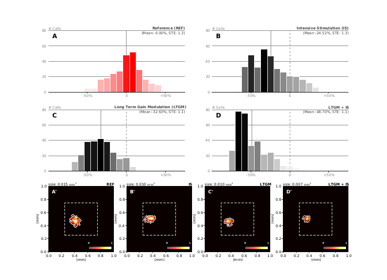
Top: histograms of relative change of receptive field sizes in the region of interest under the influence of intensive stimulation, attention and a combination of both. Bottom: receptive field of a single cell recorded at the end of each of the aforementioned experiment.
Figure 2: Relative change of receptive field sizes in the RoI compared to the reference. A. Histogram of receptive field relative sizes in the RoI after initial training (50 000 samples) without any gain modulation nor intensive stimulation. Values below zero indicate receptive field with size smaller than the mean (actual mean=0.029 mm2, std=0.0058) B. Histogram of receptive field size changes with intensive stimulation in the RoI (with a 3 to 1 ratio) using 30 000 extra samples. Values below zero indicate receptive field shrinkage. The solid vertical bar indicates the mean size change for the whole population within the RoI (actual mean=0.019 mm2, std=0.0053). C. Histogram of receptive field size changes with long term gain modulaton in the RoI using 30 000 extra samples. Values below zero indicate receptive field shrinkage. The solid vertical bar indicates the mean size change for the whole population within the RoI (actual mean=0.016 mm2, std=0.0045). D. Histogram of receptive field size changes with long term gain modulaton and intensive stimulation (with a 1/1 ratio) in the RoI using 30 000 extra samples. Values below zero indicate receptive field shrinkage. The solid vertical bar indicates the mean size change for the whole populatiuon within the RoI (actual mean=0.011 mm2, std=0.0053) Bottom row. Receptive field of a single cell recorded at the end of each of the aforementionned experiment. The receptive field size in the LTGM-IS experiment (0.010 mm2) has shrunk to one third of the reference size (0.030 mm2) while being stronger.
All the (real) data are in the http://webloria.loria.fr/~rougier/tmp/Scipy-2013/ but they’re rather big. The figure comes from a publication (in preparation) related to the self-organization of the somato-sensory cortex.
import numpy as np
import matplotlib
import matplotlib.pyplot as plt
from matplotlib.ticker import MultipleLocator, FormatStrFormatter
from mpl_toolkits.axes_grid1.inset_locator import inset_axes
from matplotlib.patches import Rectangle
import matplotlib.patheffects as PathEffects


def histogram(letter, text, Ref, X, color=(0,0,0)):

    ref_mean = np.mean(Ref)
    x_mean   = np.mean(X)
    X  =  100.0*(X - ref_mean) / ref_mean
    mean = np.mean(X)
    std = np.std(X)
    ste = std/np.sqrt(len(X))

    x_mean = 100.0*(x_mean - ref_mean) / ref_mean

    bin_size=8.0
    min_edge=-95.0
    max_edge=95.0
    N = (max_edge-min_edge)/bin_size
    bins = np.linspace(min_edge, max_edge, N+1)
    counts, bins, patches = axes.hist(X, bins=bins, facecolor=fg, edgecolor=bg, lw=1)

    n_max = float(counts.max())
    i_max = counts.argmax()
    x_max = (bins[i_max]+bins[i_max+1])/2.
    for n, patch in zip(counts,patches):
        #v = np.sqrt((1-n/n_max))
        v = (1-n/n_max)
        patch.set_facecolor( (max(v,color[0]), max(v,color[1]), max(v,color[2])))

    ymin,ymax = 0, 80
    xmin,xmax = -100, +75
    plt.xlim(xmin,xmax)
    plt.ylim(ymin,ymax+1)

    plt.axvline(x=0,ymin=ymin,ymax=ymax/(ymax+1.),
                color='0.5',lw=.75,zorder=-1,ls='--')
    plt.axvline(x=x_mean,ymin=ymin,ymax=ymax/(ymax+1.),
                color='0.5',lw=.75,zorder=-1,ls='-')

    axes.set_aspect( 0.45 * (xmax-xmin)/(ymax-ymin) )
    axes.spines['right'].set_color('none')
    axes.spines['left'].set_color('none')
    axes.spines['top'].set_color('none')
    axes.xaxis.set_ticks_position('bottom')
    axes.yaxis.set_ticks_position('left')

    plt.yticks([])
    plt.xticks([-50,0,+50],['-50%','0','+50%'])

    axes.yaxis.set_major_locator(MultipleLocator(20.0))
    axes.grid(which='major', axis='y', linewidth=0.75, linestyle='-', color='0.5')

    [t.set_color('0.5') for t in axes.xaxis.get_ticklabels()]
    [t.set_color('0.5') for t in axes.yaxis.get_ticklabels()]
    [t.set_alpha(0.0) for t in axes.yaxis.get_ticklines()]

    plt.text(xmin+5,0.95*ymax,letter, fontsize='xx-large', va='top', color=fg,weight='bold')
    plt.text(75,ymax+1,text, va='bottom',ha='right',color='.25',weight='bold')
    plt.text(75,ymax-1, '(Mean:%.2f%%, STE: %.1f)' % (mean,ste), va='top',ha='right',color='.25')
    plt.text(-100,ymax+1,"# Cells", va='bottom',ha='left',color='.5')


def imshow(letter, text, figref, Z):
    interpolation = 'bicubic'
    cmap = plt.cm.hot
    axis = plt.gca()
    vmin, vmax = 0, 1

    im = plt.imshow(Z, extent = [0,1,0,1],
                    interpolation=interpolation, cmap=cmap, vmin=0,vmax=1)
    ins = inset_axes(axis, width="35%", height="5%",  loc=4, borderpad=.5)
    cbar = plt.colorbar(cax=ins, orientation="horizontal",ticks=[vmin, vmax])
    ins.xaxis.set_ticks_position("top")
    cbar.ax.set_xticklabels(['0', '1'], fontsize=8, color='w', weight='bold')

    CS = axis.contour(Z, [0.05], origin='upper',
                      linewidths=1, colors='w', extent=(0,1,0,1))

    axis.set_xlim(0,1)
    axis.set_ylim(0,1)

    axis.xaxis.set_major_locator(MultipleLocator(0.2))
    #axis.xaxis.set_minor_locator(MultipleLocator(0.01))
    axis.yaxis.set_major_locator(MultipleLocator(0.2))
    #axis.yaxis.set_minor_locator(MultipleLocator(0.01))
    axis.get_xaxis().tick_bottom()
    axis.get_yaxis().tick_left()
    axis.set_xlabel('(mm)')
    axis.set_ylabel('(mm)')

    rect = Rectangle((.25,.25), .5, .5, facecolor='None', edgecolor='w', ls='dashed', lw=.75)
    axis.add_patch(rect)
    #t = axis.text(.26,.74, "RoI", ha='left', va='top', zorder=1,
    #               weight='bold', color='w', fontsize=16, alpha=.5)
    #t.set_path_effects([PathEffects.withStroke(linewidth=.75,foreground="k",alpha=.25)])
    axis.text(1,1.01,text, ha='right', va='bottom', weight='bold')
    axis.text(0,1.01,letter, ha='left', va='bottom', color='k')

    axis.text(0.05,0.95,figref, ha='left', va='top', color='w',  weight='bold', fontsize=16)


    return im


if __name__ == '__main__':

    REF    = np.load('./REF-ROI-sizes.npy')
    STGM   = np.load('./STGM-ROI-sizes.npy')
    LTGM   = np.load('./LTGM-ROI-sizes.npy')
    IS     = np.load('./IS-ROI-sizes.npy')
    LTGMIS = np.load('./LTGMIS-ROI-sizes.npy')

    s = 1/(64.0*64.0)
    print "REF:    mean=%.3f, std=%.4f" % (s*np.mean(REF),    s*np.std(REF))
    print "STGM:   mean=%.3f, std=%.4f" % (s*np.mean(STGM),   s*np.std(STGM))
    print "IS:     mean=%.3f, std=%.4f" % (s*np.mean(IS),     s*np.std(IS))
    print "LTGM:   mean=%.3f, std=%.4f" % (s*np.mean(LTGM),   s*np.std(LTGM))
    print "LTGMIS: mean=%.3f, std=%.4f" % (s*np.mean(LTGMIS), s*np.std(LTGMIS))


    fg = 0.0,0.0,0.0
    bg = 1.0,1.0,1.0
    #matplotlib.rcParams['ytick.major.size'] = 0
    #matplotlib.rcParams['ytick.minor.size'] = 9
    matplotlib.rcParams['xtick.major.width'] = .5
    matplotlib.rcParams['ytick.major.width'] = .5
    matplotlib.rcParams['xtick.direction'] = 'out'
    matplotlib.rcParams['ytick.direction'] = 'out'
    matplotlib.rcParams['font.size'] = 12.0
    matplotlib.rc('axes', facecolor = bg)
    matplotlib.rc('axes', edgecolor = fg)
    matplotlib.rc('xtick', color = fg)
    matplotlib.rc('ytick', color = fg)
    matplotlib.rc('figure', facecolor = bg)
    matplotlib.rc('savefig', facecolor = bg)

    fig = plt.figure(figsize=(18,13), dpi=72)
    axes = plt.subplot(321, axisbelow=True)
    histogram("A","Reference (REF)", REF,REF,color=(1,0,0))
    axes = plt.subplot(322, axisbelow=True)
    histogram("B","Intensive Stimulation (IS)", REF,IS)
    axes = plt.subplot(323, axisbelow=True)
    histogram("C","Long Term Gain Modulation (LTGM)", REF,LTGM)
    axes = plt.subplot(324, axisbelow=True)
    histogram("D","LTGM + IS", REF,LTGMIS)


    REF = np.load('./model_response_64_ref.npy')
    IS = np.load('./model_response_64_is.npy')
    LTGM = np.load('./model_response_64_ltgm.npy')
    STGM = np.load('./model_response_64_stgm.npy')
    LTGMIS = np.load('./model_response_64_ltgm_is.npy')

    x,y = 20,1
    RF_REF    = REF[x::32,y::32]
    RF_IS     = IS[x::32,y::32]
    RF_LTGM   = LTGM[x::32,y::32]
    RF_LTGMIS = LTGMIS[x::32,y::32]

#    print (RF_REF>0).sum()/ float(64*64)
#    print (RF_IS>0).sum()/ float(64*64)
#    print (RF_LTGM>0).sum()/ float(64*64)
#    print (RF_LTGMIS>0).sum()/ float(64*64)

    Z = np.abs(RF_REF) + np.abs(RF_IS) + np.abs(RF_LTGM) + np.abs(RF_LTGMIS)
    X = np.argwhere(Z.sum(axis=1) >= 0.0)
    xmin,xmax = X.min(), X.max()+1
    Y = np.argwhere(Z.sum(axis=0) >= 0.0)
    ymin,ymax = Y.min(), Y.max()+1

    plt.subplot(3,4,9,aspect=1)
    imshow("size: %.3f $\mathrm{mm}^\mathrm{2}$" % ((RF_REF>0).sum()/ float(64*64)),
           "REF","A'",RF_REF[xmin:xmax,ymin:ymax])
    plt.subplot(3,4,10,aspect=1)
    imshow("size: %.3f $\mathrm{mm}^\mathrm{2}$" % ((RF_IS>0).sum()/ float(64*64)),
           "IS","B'",RF_IS[xmin:xmax,ymin:ymax])
    plt.subplot(3,4,11,aspect=1)
    imshow("size: %.3f $\mathrm{mm}^\mathrm{2}$" % ((RF_LTGM>0).sum()/ float(64*64)),
           "LTGM", "C'", RF_LTGM[xmin:xmax,ymin:ymax])
    plt.subplot(3,4,12,aspect=1)
    im = imshow("size: %.3f $\mathrm{mm}^\mathrm{2}$" % ((RF_LTGMIS>0).sum()/ float(64*64)),
                "LTGM + IS", "D'", RF_LTGMIS[xmin:xmax,ymin:ymax])

    # ax = plt.gca()
    # axins = inset_axes(ax,
    #                    width="5%", # width = 10% of parent_bbox width
    #                    height="100%", # height : 50%
    #                    loc=3,
    #                    bbox_to_anchor=(1.05, 0., 1, 1),
    #                    bbox_transform=ax.transAxes,
    #                    borderpad=0 )
    # plt.colorbar(im, cax=axins, ticks=[0,1])

    plt.savefig("size-histogram.pdf")
    plt.show()


