Adrian Price-Whelan
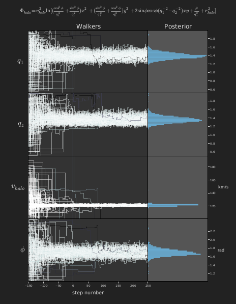
Visualization of MCMC chains (walkers; left panels) and derived posterior probability distributions (right panels) for four parameters in the specified dark matter halo potential model. The model is evaluated against simulated observations of RR Lyrae in the Sagittarius stream. Steps -150 to 0 were considered burn-in and rejected from the displayed posteriors.
"""
    Make a figure to visualize using MCMC (in particular, the Python package
    emcee) to infer 4 parameters from a parametrized model of the Milky Way's
    dark matter halo by using tracer stars from the Sagittarius Stream.

    If you're unfamiliar with the jargon here (walkers, Sgr, etc.), check out:
        - Law & Majewski 2010
            http://iopscience.iop.org/0004-637X/714/1/229/pdf/apj_714_1_229.pdf
        - emcee
            http://dan.iel.fm/emcee/
        - Ensemble samplers with affine-invariance
            http://msp.org/camcos/2010/5-1/camcos-v5-n1-p04-p.pdf

"""

# Standard library
import cPickle as pickle

# Third-party dependencies
import astropy.units as u
import matplotlib
import matplotlib.pyplot as plt
import matplotlib.cm as cm
import matplotlib.gridspec as gridspec
import numpy as np

matplotlib.rcParams['font.family'] = "sans-serif"
font_color = "#dddddd"
tick_color = "#cdcdcd"

# Map the codified parameter names to their sexy latex equivalents
param_to_latex = dict(q1=r"$q_1$",
                      qz=r"$q_z$",
                      v_halo=r"$v_{halo}$",
                      phi=r"$\phi$")

halo_params = ["q1", "qz", "v_halo", "phi"]
acceptance_fractions, flat_chain, chain = pickle.load(open("2013-03-12_05-03-29_q1_qz_v_halo_phi_w200_s400.pickle"))
chain = chain[(acceptance_fractions > 0.15) & (acceptance_fractions < 0.6)]

# Create a figure object with same aspect ratio as a sheet of paper...
fig = plt.figure(figsize=(16,20.6))

# I want the plot of individual walkers to span 2 columns
gs = gridspec.GridSpec(4, 3)

# The halo velocity (v_halo) parameter is stored in units of kpc/Myr, but I
#   want to plot it in km/s
for xx in range(chain.shape[0]):
    for yy in range(chain.shape[1]):
        chain[xx,yy,2] = (chain[xx,yy,2]*u.kpc/u.Myr).to(u.km/u.s).value

# I could compute this, but for now I just hard code it by looking at the
#   plots by eye...
converged_idx = 150

# For each parameter, I want to plot each walker on one panel, and a histogram
#   of all links from all walkers past 150 steps (approximately when the chains
#   converged)
for ii,param in enumerate(halo_params):
    these_chains = chain[:,:,ii]

    # I'm going to color the walkers by their variance past the bulk convergence
    #   point, so here I compute the maximum variance to scale the others to 0-1
    max_var = max(np.var(these_chains[:,converged_idx:], axis=1))

    ax1 = plt.subplot(gs[ii, :2])
    ax1.set_axis_bgcolor("#333333")

    ax1.axvline(0,
                color="#67A9CF",
                alpha=0.7,
                linewidth=2)

    for walker in these_chains:
        ax1.plot(np.arange(len(walker))-converged_idx, walker,
                drawstyle="steps",
                color=cm.bone_r(np.var(walker[converged_idx:]) / max_var),
                alpha=0.5)

    ax1.set_ylabel(param_to_latex[param],
                   fontsize=36,
                   labelpad=18,
                   rotation="horizontal",
                   color=font_color)

    # Don't show ticks on the y-axis
    ax1.yaxis.set_ticks([])

    # For the plot on the bottom, add an x-axis label. Hide all others
    if ii == len(halo_params)-1:
        ax1.set_xlabel("step number", fontsize=24, labelpad=18, color=font_color)
    else:
        ax1.xaxis.set_visible(False)

    ax2 = plt.subplot(gs[ii, 2])
    ax2.set_axis_bgcolor("#555555")

    # Create a histogram of all values past the converged point. Make 100 bins
    #   between the y-axis bounds defined by the 'walkers' plot.
    ax2.hist(np.ravel(these_chains[:,converged_idx:]),
             bins=np.linspace(ax1.get_ylim()[0],ax1.get_ylim()[1],100),
             orientation='horizontal',
             facecolor="#67A9CF",
             edgecolor="none")

    # Same y-bounds as the walkers plot, so they line up
    ax1.set_ylim(np.min(these_chains[:,0]), np.max(these_chains[:,0]))
    ax2.set_ylim(ax1.get_ylim())
    ax2.xaxis.set_visible(False)
    ax2.yaxis.tick_right()

    # For the first plot, add titles and shift them up a bit
    if ii == 0:
        t = ax1.set_title("Walkers", fontsize=30, color=font_color)
        t.set_y(1.01)
        t = ax2.set_title("Posterior", fontsize=30, color=font_color)
        t.set_y(1.01)

    if param == "v_halo":
        ax2.set_ylabel("km/s",
                       fontsize=20,
                       rotation="horizontal",
                       color=font_color,
                       labelpad=16)
    elif param == "phi":
        ax2.set_ylabel("rad",
                       fontsize=20,
                       rotation="horizontal",
                       color=font_color,
                       labelpad=16)
    ax2.yaxis.set_label_position("right")

    # Adjust axis ticks, e.g. make them appear on the outside of the plots and
    #   change the padding / color.
    ax1.tick_params(axis='x', pad=2, direction='out', colors=tick_color, labelsize=14)
    ax2.tick_params(axis='y', pad=2, direction='out', colors=tick_color, labelsize=14)

    # Removes the top tick marks
    ax1.get_xaxis().tick_bottom()

    # Hack because the tick labels for phi are wonky... but this removed the
    #   first and last tick labels so I can squash the plots right up against
    #   each other
    if param == "phi":
        ax2.set_yticks(ax2.get_yticks()[1:-2])
    else:
        ax2.set_yticks(ax2.get_yticks()[1:-1])

# Effing long equation for the logarithmic halo potential with a possible
#   rotation relative to the MW disk.
fig.suptitle(r"$\Phi_{halo} = v_{halo}^2 \ln[(\frac{\cos^2\phi}{q_1^2}+\frac{\sin^2\phi}{q_2^2})x^2 + (\frac{\sin^2\phi}{q_1^2}+\frac{\cos^2\phi}{q_2^2})y^2 + 2\sin\phi\cos\phi(q_1^{-2}-q_2^{-2})xy + \frac{z^2}{q_z^2} + r_{halo}^2]$", fontsize=26, color=font_color)
fig.subplots_adjust(hspace=0.0, wspace=0.0, bottom=0.075, top=0.9, left=0.12, right=0.88)
plt.savefig("walkers.pdf", facecolor='#222222')


