Kristen Thyng
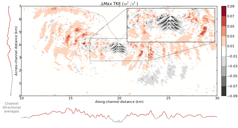
This figure is from a paper for the European Wave and Tidal Energy Conference (EWTEC) that I am working on with a co-author. The paper describes a study we did together combining a simulation of an idealized tidal channel with a symmetric headland in the middle and an array of ten turbines near the headland. This combination of efforts allows us to start to understand the effects of turbines on increasingly realistic flows, both near the turbine array and farther field, kilometers away down the channel.
The plot shows the difference in maximum turbulent kinetic energy (TKE) between a simulation with no turbines and a simulation with an array of turbines. Positive (red) values indicate areas in which the initial case has larger maximum values and negative (grey) values indicate areas in which the turbine array case has larger values. Line plots to the left (bottom) of the main plot area show the along- (across-) channel average of the plot values, with coloring indicating position greater than (red) or less than (grey) zero.
There is a distinction in relative behavior in the cases in the near- and far-field. Very near to the turbines and in their wake, the TKE is stronger in the turbine case, which is expected given that several terms have been added to the turbulence equations in order to model the effect of the turbines. Further downstream, the initial, no turbine case TKE is larger than the turbine case, probably due to the dissipation due to the turbines in the regular array case. These trends are reflected in the along- and across-channel averages shown alongside the plot: the initial case tends to be larger except near the turbines themselves.
Source
import plot_gen as pg
import numpy as np

# # Some subtraction plots
# # vorticity (da)
# # levels = np.linspace(-.09,.09,10)
# smax: np.linspace(-.9,.9,10), smean: np.linspace(-.45,.45,10)
# zetamax: np.linspace(-.01,.01,9)
var = {'vort':{'levels':np.linspace(-.0045,.0045,10),'colormap':'RdGy_r','title':r'$\Delta$Max vertical vorticity $(1/s)$'},
	   'tke':{'levels':np.linspace(-.09,.09,10),'colormap':'RdGy_r','title':r'$\Delta$Max TKE ($m^2/s^2$)'},
	   'w':{'levels':np.linspace(-.9,.9,10),'colormap':'RdGy_r','title':r'$\Delta$Max vertical velocity $(m/s)$'},
	   's':{'levels':np.linspace(-.9,.9,10),'colormap':'RdGy_r','title':r'$\Delta$Max horizontal speed $(m/s)$'},
	   'zeta':{'levels':np.linspace(-.0001,.0001,9),'colormap':'RdGy_r','title':r'$\Delta$Mean zeta $(m)$'},
	   'mkpd':{'levels':np.linspace(-.9,.9,10),'colormap':'RdGy_r','title':r'$\Delta$ mean kinetic power density $(kW/m^2)$'},
	   'abi':{'levels':np.linspace(-27,27,10),'colormap':'RdGy_r','title':r'$\Delta$ asymmetry (degrees)'},
	   'stdbi':{'levels':np.linspace(-27,27,10),'colormap':'RdGy_r','title':r'$\Delta$ directional deviation (degrees)'}}

name = 'tke' # when i want to do more do a loop
oper = 'max' # operation (max, mean, metric, min,gradmean)
zoom = 'zmid'
# vlevel = 'hubheight' #'surface'#'hubheight' (depth-averaged)
data = np.load('diff.npz')
diff = data['diff']
x = data['x']
y = data['y']
mask = data['mask']
data.close()

### TEMP
# ind = np.arange(0,50)#15,15+25) # half the cycle

# diff = d.max(axis=0)-dr.max(axis=0)

pg.plt(x/1000.,y/1000.,diff,mask,zoom,
	var[name]['colormap'],var[name]['levels'],
	name + oper + '.pdf',
	var[name]['title'])
'''
troc_plot_gen.py
Kristen M. Thyng
November 2012

Plot properties that were saved and calculated in troc_calc.py, at
multiple depths. More general than troc_plot.py.

Movies:
	Density
	U Velocity
	V Velocity
	TKE (5 m down)
	Vertical Velocity (5 m down)
	Free Surface
Plots:
	Asymmetry properties:
		bidirectionality
		directional deviation
	Vorticity (need to calculate in sigma coordinates)
	Mean speed
	Mean Density
	Mean TKE
	Mean w
	Mean vorticity
	Mean kinetic power density
	Mean free surface
	Free surface signal at edge of domain

'''

# import matplotlib
# matplotlib.use("Agg") # set matplotlib to use the backend that does not require a windowing system
import os
import numpy as np
from matplotlib.pyplot import *
import matplotlib.colors as colors
from matplotlib import rc, ticker, cm
import troc_calc as tr
import pdb
import op
import netCDF4 as netCDF
from pylab import *
from mpl_toolkits.axes_grid1.inset_locator import zoomed_inset_axes
from mpl_toolkits.axes_grid1.inset_locator import mark_inset

#rc('text', usetex=True) # for latex rendering
##rc('font', family='serif')

# # User stuff
# var = 'mssurface'
# vtype = 'calculate'
# zoom = 'zout'
# xlims = (0,40)
# ylims = (0,7)

hgrey = '#737373'
hred = '#c94741'

def plt(x,y,z,mask,zoom,colormap,levels,fname,Title):

	if zoom == 'zout':
		xlims = (0,40)
		ylims = (0,7)
		dy = 24
		dx = 18
		ms = 1.5
	elif zoom == 'zmid':
		xlims = (10,30)
		ylims = (0,7)
		dy = 24
		dx = 14
		ms = 1.5 # min shaft length
	elif zoom == 'zin':
		xlims = (17,23)
		ylims = (3,5)
		dy = 12#6
		dx = 8#4
		ms = .25

	# Make plots
	# rc('text',usetex=True)
	matplotlib.rcParams.update({'font.size': 16})
	# if vtype == 'calculate':
		# if var == 'abisurface' or var == 'abihubheight' or var == 'stdbisurface' or var == 'stdbihubheight':
		# 	figure(figsize=(18,6))
		# 	contourf(x,y,d,[5,10,15,20,25,30,35,40],cmap=colormap)#,vmin=dmin,vmax=dmax)
		# 	xlim(xlims)
		# 	ylim(ylims)
		# 	colorbar()
		# 	xlabel('Along-channel distance (km)')
		# 	ylabel('Across-channel distance (km)')
		# 	title(Title)
		# 	savefig('figures/calculate/' + var + zoom + '.png',bbox_inches='tight')
		# 	close()
		# else:
	# figure(figsize=(18,6))

	# definitions for axes, a la http://matplotlib.org/examples/pylab_examples/scatter_hist.html
	left, bottom = 0.05, 0.1 # for very left and very bottom
	thickx, thicky = 0.03, 0.125 # thickness of the left and bottom plots
	width, height = 0.75, 0.6 # width and height of main plot
	dpx = .025 # space between plots
	dpy = .08

	# axes for each of the three plots: [left,bottom,width,height]
	rect_main = [left+thickx+dpx,bottom+thicky+dpy,width+.153,height] # main plot
	rect_left = [left,bottom+thicky+dpy,thickx,height] # left side small plot
	rect_bottom = [left+thickx+dpx,bottom,width,thicky] # bottom small plot
	nullfmt   = NullFormatter()         # no labels
	nullloc   = NullLocator()

	# start with a rectangular figure
	figure(1,figsize=(18,10))#18,6))

	axMain = axes(rect_main)

	# main plot

	# pcolormesh(x,y,z,cmap=colormap)#,vmin=dmin,vmax=dmax)
	# cmap = cm.PRGn
	# levels=[-0.08      , -0.06222222, -0.04444444, -0.02666667, -0.00888889,
 #        0.00888889,  0.02666667,  0.04444444,  0.06222222,  0.08]
 	# dmax = np.max(z.max(),abs(z.min()))
	# this is to prevent the whiting out of larger values in the contour maps
	dmax = np.max(levels)
	ind = (z>=dmax)
	z[ind] = dmax
	ind = (z<=-dmax)
	z[ind] = -dmax
	# pdb.set_trace()
	contourf(x,y,z,levels,cmap=get_cmap(colormap))#levels=np.linspace(-dmax,dmax,10))#,levels=np.linspace(-.09,.09,10))#cmap=cm.get_cmap(colormap, len(levels)-1))#cmap=colormap)#,vmin=dmin,vmax=dmax#levels=np.linspace(dmin,dmax,9))
	# pcolormesh(x,y,z,cmap=colormap,vmin=-dmax,vmax=dmax)
	colorbar(pad=.02)
	#set_cmap(colormap)

	axMain.set_xlim(xlims)
	axMain.set_ylim(ylims)
	axMain.set_title(Title)
	axMain.set_ylabel('Across-channel distance (km)')
	axMain.set_xlabel('Along-channel distance (km)')
	# axMain.xaxis.set_major_formatter(nullfmt) # no labels
	# axMain.yaxis.set_major_formatter(nullfmt) # no labels

	# Draw in headland to distinguish from the flow in whiter plots
	hold('on')
	contour(x,y,mask,levels=[0],colors='grey',alpha=.5)
	# ind = (mask == 0)
	# pcolor(x,y,ind*.5)

	# Try including various averages along the edges of the plots: left and bottom
	# Left plot: averaged along-channel
	axLeft = axes(rect_left,frameon=False)#,sharey=axMain)
	ind = ~np.isnan(z)
	# pdb.set_trace()
	# zacross = z.mean(axis=1)
	# poor man's nanmean
	zacross = np.nansum(z,axis=1)/ind.sum(axis=1)
	indp = (zacross>0)
	indn = (zacross<=0)
	zacrossp = zacross.copy()
	zacrossp[indn] = np.nan
	zacrossn = zacross.copy()
	zacrossn[indp] = np.nan
	axLeft.plot(zacrossp,y[:,0],color=hred,alpha=1,linewidth=2)
	hold('on')
	# ind = (zacross<=0)
	axLeft.plot(zacrossn,y[:,0],color=hgrey,alpha=.7,linewidth=2)
	# axLeft.plot(np.zeros(y.shape[0]),y[:,0],':k')
	xmax = max(zacross.max(),abs(zacross.min()))
	axLeft.set_xlim((xmax,-xmax))
	axLeft.set_ylim(ylims)
	axLeft.set_xlabel('\n\n Channel\n Directional\n averages',color=hgrey)
	# locs,labels = xticks()
	# setp(labels,visible=False)#rotation=90,color='grey')
	# setp(locs,visible=False)#rotation=90,color='grey')
	axLeft.yaxis.set_major_locator(nullloc) # no labels
	axLeft.xaxis.set_major_locator(nullloc) # no labels

	# Bottom plot: averaged across-channel
	axBottom = axes(rect_bottom,frameon=False)#,sharex=axMain)
	zalong = z.mean(axis=0)
	indp = (zalong>0)
	indn = (zalong<=0)
	zalongp = zalong.copy()
	zalongp[indn] = np.nan
	zalongn = zalong.copy()
	zalongn[indp] = np.nan
	axBottom.plot(x[0,:],zalongn,color=hgrey,alpha=.7,linewidth=2)
	hold('on')
	axBottom.plot(x[0,:],zalongp,color=hred,alpha=1,linewidth=2)
	# axBottom.plot(x[0,:],np.zeros(x.shape[1]),':k')
	axBottom.set_xlim(xlims)
	ymax = max(zalong.max(),abs(zalong.min()))
	axBottom.set_ylim((-ymax,ymax))
	axBottom.yaxis.set_major_locator(nullloc) # no labels
	axBottom.xaxis.set_major_locator(nullloc) # no labels
	# axBottom.yaxis.tick_right()

	# Inset magnified plot
	# Inset image
	axins = zoomed_inset_axes(axMain,1.5,loc=1) # zoom=6
	# pcolormesh(x,y,d[i,:,:],cmap=colormap,vmin=dmin,vmax=dmax)
	# pcolormesh(x,y,z,cmap=colormap,vmin=-dmax,vmax=dmax)
	contourf(x,y,z,levels,cmap=get_cmap(colormap))
	hold('on')
	contour(x,y,mask,levels=[0],colors='grey',alpha=.5)
	# clabel(C,fontsize=14,fmt='%2.1f')#,manual=True)
	# subregion of the original image
	x1,x2,y1,y2 = 17,23,2.75,4.5
	axins.set_xlim(x1,x2)
	axins.set_ylim(y1,y2)
	xticks(visible=False)
	yticks(visible=False)
	setp(axins,xticks=[],yticks=[])
	# draw a bbox of the region of the inset axes in the parent axes and
	# connecting lines between the bbox and the inset axes area
	mark_inset(axMain, axins, loc1=2, loc2=4, fc="none", ec="0.5")
	draw()
	show()


	# title(Title)
	savefig(fname,bbox_inches='tight')
	# savefig('figures/' + var + zoom + '.png',bbox_inches='tight')
	show()
	# close()


