Entry 3 (Third Place)¶

Authors¶

Jake Vanderplas

Zeljko Ivezic

Andrew Connolly

This figure is based on data presented in figures 3-4 of Parker & Ivezic et al (2008). A similar figure appears in the book “Statistics, Data Mining, and Machine Learning in Astronomy”, by Ivezic, Connolly, Vanderplas, and Gray (2013).

Running this code requires astroML, a lightweight python package which can be quickly installed using pip install astroML. See http://astroML.github.com for more information. AstroML will automatically download and cache the required dataset to $HOME/astroML_data.

Figure Caption¶

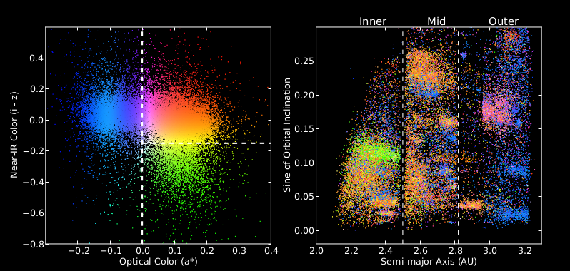
These panels visualize a 4-dimensional correlation between orbits and surface color for about 35,000 main-belt asteroids (found between Mars and Jupiter) observed by the Sloan Digital Sky Survey. The left panel quantifies the variation of the asteroid surface chemistry using two measured colors: a* is an optical color (as would be seen by e.g. human eyes) and i-z is a near-infrared color (as would be seen by e.g. snake eyes). The dots corresponding to individual objects are color-coded according to the object’s position in this diagram. Blue shades are representative of carbonaceous surfaces, and orange and green shades correspond to silicate surfaces. The right panel is constructed with two orbital parameters: semi-major axis a (AU stands for astronomical unit, equal to Sun-Earth distance) and sine of the orbital inclination i. The vertical dashed lines mark the so-called Kirkwood gaps, where no objects are found because of resonant gravitational scattering due to Jupiter. These gaps define the three main-belt zones. The easily discernible clusters of points correspond to the so-called orbital families of asteroids, believed to be smaller remnants of larger objects destroyed in collisions. The dots corresponding to individual objects are color-coded according to the two-dimensional color palette from the left panel and the measured surface colors. The vividly demonstrated fact that orbitally related asteroids also have similar colors (and therefore similar surface chemistry) is evidence that asteroids in these families share a common origin.

Products¶

PDF

Source¶

import numpy as np
from matplotlib import pyplot as plt
from astroML.datasets import fetch_moving_objects
from astroML.plotting.tools import devectorize_axes


def black_bg_subplot(*args, **kwargs):
    """Create a subplot with black background"""
    kwargs['axisbg'] = 'k'
    ax = plt.subplot(*args, **kwargs)

    # set ticks and labels to white
    for spine in ax.spines.values():
        spine.set_color('w')

    for tick in ax.xaxis.get_major_ticks() + ax.yaxis.get_major_ticks():
        for child in tick.get_children():
            child.set_color('w')

    return ax


def compute_color(mag_a, mag_i, mag_z, a_crit=-0.1):
    """
    Compute the scatter-plot color using code adapted from
    TCL source used in Parker 2008.
    """
    # define the base color scalings
    R = np.ones_like(mag_i)
    G = 0.5 * 10 ** (-2 * (mag_i - mag_z - 0.01))
    B = 1.5 * 10 ** (-8 * (mag_a + 0.0))

    # enhance green beyond the a_crit cutoff
    G += 10. / (1 + np.exp((mag_a - a_crit) / 0.02))

    # normalize color of each point to its maximum component
    RGB = np.vstack([R, G, B])
    RGB /= RGB.max(0)

    # return an array of RGB colors, which is shape (n_points, 3)
    return RGB.T


#------------------------------------------------------------
# Fetch data and extract the desired quantities
data = fetch_moving_objects(Parker2008_cuts=True)
mag_a = data['mag_a']
mag_i = data['mag_i']
mag_z = data['mag_z']
a = data['aprime']
sini = data['sin_iprime']

# dither: magnitudes are recorded only to ± 0.01
mag_a += -0.005 + 0.01 * np.random.random(size=mag_a.shape)
mag_i += -0.005 + 0.01 * np.random.random(size=mag_i.shape)
mag_z += -0.005 + 0.01 * np.random.random(size=mag_z.shape)

# compute RGB color based on magnitudes
color = compute_color(mag_a, mag_i, mag_z)

#------------------------------------------------------------
# set up the plot
fig = plt.figure(figsize=(10.5, 5), facecolor='k')
fig.subplots_adjust(left=0.08, right=0.95, wspace=0.2,
                    bottom=0.1, top=0.9)

# plot the color-magnitude plot
ax = black_bg_subplot(121)
ax.scatter(mag_a, mag_i - mag_z,
           c=color, s=1, lw=0, edgecolors=color)

# uncomment to convert SVG points to pixels
#devectorize_axes(ax, dpi=400)

ax.plot([0, 0], [-0.8, 0.6], '--w', lw=2)
ax.plot([0, 0.4], [-0.15, -0.15], '--w', lw=2)

ax.set_xlim(-0.3, 0.4)
ax.set_ylim(-0.8, 0.6)

ax.set_xlabel('Optical Color (a*)', color='w')
ax.set_ylabel('Near-IR Color (i - z)', color='w')

# plot the orbital parameters plot
ax = black_bg_subplot(122)
ax.scatter(a, sini,
           c=color, s=1, lw=0, edgecolors=color)

# uncomment to convert SVG points to pixels
#devectorize_axes(ax, dpi=400)

ax.plot([2.5, 2.5], [-0.02, 0.3], '--w')
ax.plot([2.82, 2.82], [-0.02, 0.3], '--w')

ax.set_xlim(2.0, 3.3)
ax.set_ylim(-0.02, 0.3)

ax.set_xlabel('Semi-major Axis (AU)', color='w')
ax.set_ylabel('Sine of Orbital Inclination', color='w')

# label the plot
text_kwargs = dict(color='w', fontsize=14,
                   transform=plt.gca().transAxes,
                   ha='center', va='bottom')

ax.text(0.25, 1.01, 'Inner', **text_kwargs)
ax.text(0.53, 1.01, 'Mid', **text_kwargs)
ax.text(0.83, 1.01, 'Outer', **text_kwargs)

# Saving the black-background figure requires some extra arguments:
fig.savefig('asteroids.pdf',
            facecolor='black',
            edgecolor='none')

plt.show()

Python source